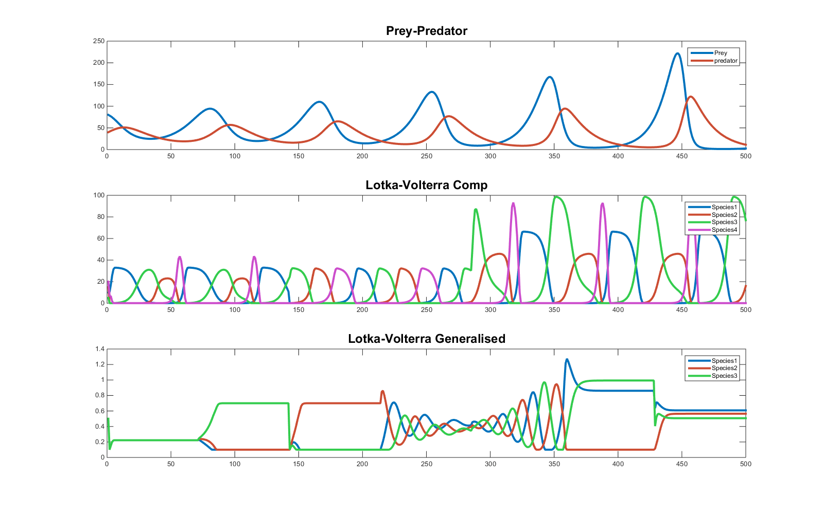
Lotka-Volterra equations have been first developed to simulate ecological nonlinear interactions among different species. Assuming two species affect each another in a prey-predator relationship, basic Lotka-Volterra equations describe the fluctuation in number of the population of both species as follows:
\[ \frac{dx}{dt} = \alpha x – \beta xy \]
\[ \frac{dy}{dt} = – \gamma y \ + \delta xy \]
where x and y respectively represent prey and predator, and ẋ and ẏ denote the growth rate of each population over time (t). The interaction is regulated by four parameters α, β, γ and δ. The population of the preys x increases at a rate α and decreases as a function of both a parameter β and the dimension of both populations of preys and predators (so that an increase in predators limits the number of preys). The populations of predators increases as a function of the parameter δ and the number of elements in both species, whereas the number of predators decreases at a rate regulated by γ, simulating a constant decline in population in the absence of preys.
Interestingly, the interaction can lead to extinction of one of the two populations (x=0 or y=0). The way the equations are built do not allow for recovery of the extinct species under this condition. To avoid this problem, a minimum value can be set of either or both populations. In the script you will find at the end of this text, the minimum is set to 0, but it can be increased arbitrarily (see function lotkavolterrapp.m).
In a second example multiple populations compete for limited resources and prey one another. The populations number of all species is now described as a single vector of dimension i: the resulting interactions are characterised as follows:
\[ \frac{dx_i}{dt} = r_i x_i \Bigg(1 – \frac{\sum_j \alpha_{ij} x_j}{K_i} \Bigg) \]
Where the population of species ( x_i ) increases depending on a growth rate ( r_i )and it is affected by the presence of competing species, depending on the value of the interaction matrix α. ( K_i ) represents a carrying capacity, per species, and for simplicity it can be pulled into the interaction matrix. Note that, in the generalised version of Lotka-Volterra equations, single values in both r and α can become negative, to express natural population decrease and mutualism, respectively.
Finally, for the third example I decided to test whether these functions could be used also to simulate choice behaviour in a hypothetical task with multiple competing options (e.g. non-stationary multi-armed bandit). These equations have been designed to allow for an initial input which is used to determine the starting populations. Apart from this setting, the interaction among species is the only element that determines their numerical changes. Conversely, in a standard task with competing options, beliefs about the preferred choice change as a function of accumulated evidence or experienced feed-backs (e.g. probabilistic outcomes assigned after selecting one among multiple options). This continuous flow of information has to be included in the equations in order to bias the competition among the available choices. For instance, if in a 3 choice task (A, B and C) a participant collects sufficient information to convince herself that option A has to be favoured in comparison with option B or C, this information has to be used at each step in order to increase the value (or belief about value) associated with option A, in the Lotka-Volterra simulation of the target behavior. To accomplish this goal, I have used a solution proposed by Zhang et al. 2014 (see: ZG Control of Populations of Lotka-Volterra Equations Using Interaction Coefficients as Inputs), dynamically targeting the parameters in the main diagonal of the α matrix, which control the self-interaction of each species, thus limiting their growth. The results can be observed in the third row of the figure below, when these parameters are changed under different condition of interaction and α matrix, resulting in attractor stable states or pattern generation.
You can download the examples of parameters configuration and the function controlling the Lotka Volterra interaction here: Lotka-Volterra