
As part of the Computational Psychiatry summer (pre) course, I have discussed the differences in the approaches characterising Reinforcement learning (RL) and Bayesian models (see slides 22 onward, here: Fiore_Introduction_Copm_Psyc_July2019 ).
In particular, I have presented a case in which values can be misleading, as the correct (optimal) choice selection leads to either +100 points (75%) or -50 points (25%), whereas the suboptimal choice leads to -100 points (75%) or +50 points (25%). For instance, let’s consider an agent that has figured out which choice is optimal, but has to deal with a reversal of the value associations (in the following example, it takes place at trial n. 5 and 9):
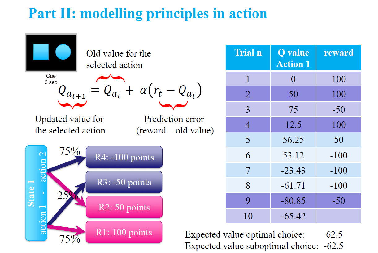 In this example, a participant who has figured out the structure of the rewards would understand that the reward received after the fifth choice (value=50) is actually indicative of the need to change action selection. As a consequence, the participant would change choice selection, while a (very simple) RL learning model would require some extra information (i.e. a series of negative values) to update its value function and adapt.
Conversely, a Bayesian model would rely only on the information as evidence that either confirms or conflicts with the existing prior/beliefs, independent of the value.
In terms of finding a solution for an artificial agent, there are ways around this problem. For instance, the RL model that can rely on a Model-Based component to keep track of the structure of rewards or it can play with learning rate values to speed up the process of the reversal learning. However, this example illustrates well how different formal descriptions of behaviour rely on significantly different assumptions and therefore may lead to significantly different interpretations. This difference becomes even more obvious if we compare the two models in an effort to match actual human behaviour.
You can download here two simple examples. The first compares the performance of the two models in searching for an optimal behaviour in a (very simple) world with two available options and stochastic feedback, as in the slide example (run the file RL_Bayes_comparison.m). The second is meant to illustrate how the two model can be used to perform a regression of parameters, to match behaviour from actual subject (run the file RL_Bayes_regression.m). In this case, the behaviour has been generated in previous iterations of the two models (so it serves as a test for parameter recovery, in a way) and the behaviour of one of the 5 agents stored in the file Agent_behaviour.mat is actually just a series of random choice selection, to be used as a comparison (you should be able to spot it out as soon as you have the results of the regression with the error)