
NB In this example I use most of the code and concepts already presented when explaining simple time series regressions using genetic algorithms. Please refer to that text for the basic explanations.
In the previous example we were happy with the idea to get rid of many features in the target time series that were considered unimportant. This may be a good solution if we consider small fluctuation as the result of noise that must be ignored to extract the correct features concerning the trends. The clear disadvantage of this strategy is that, besides noise, the regression will also potentially ignore features which may be significant. Consider for example the fluctuations expressed in these target time series:
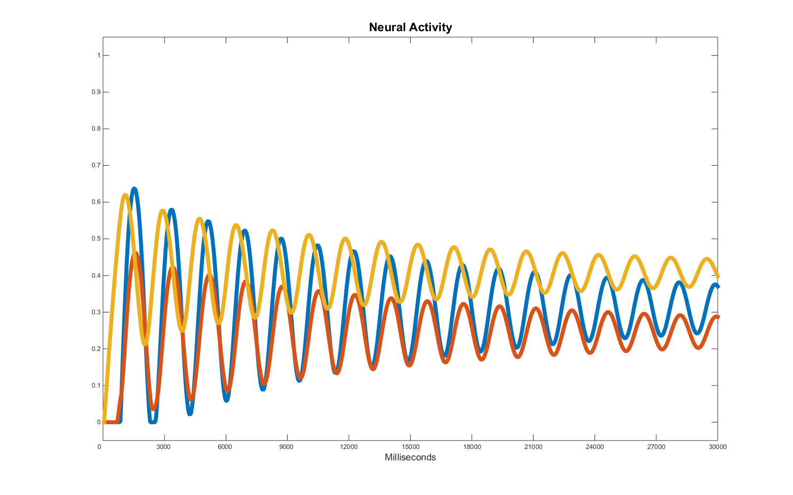
Here we have wave patterns characterised by a period, an amplitude and a central line which is important to replicate if we want a fine grain prediction of the evolution of these activities or if we are trying to understand the causal relations among each node in a network (e.g. in studies estimating the effective connectivity).
Once again then I use in this example a genetic algorithm as a regression tool. Unfortunately, if we rely on a simple distance from the target to estimate the error (as in the previous example), the result is not acceptable:
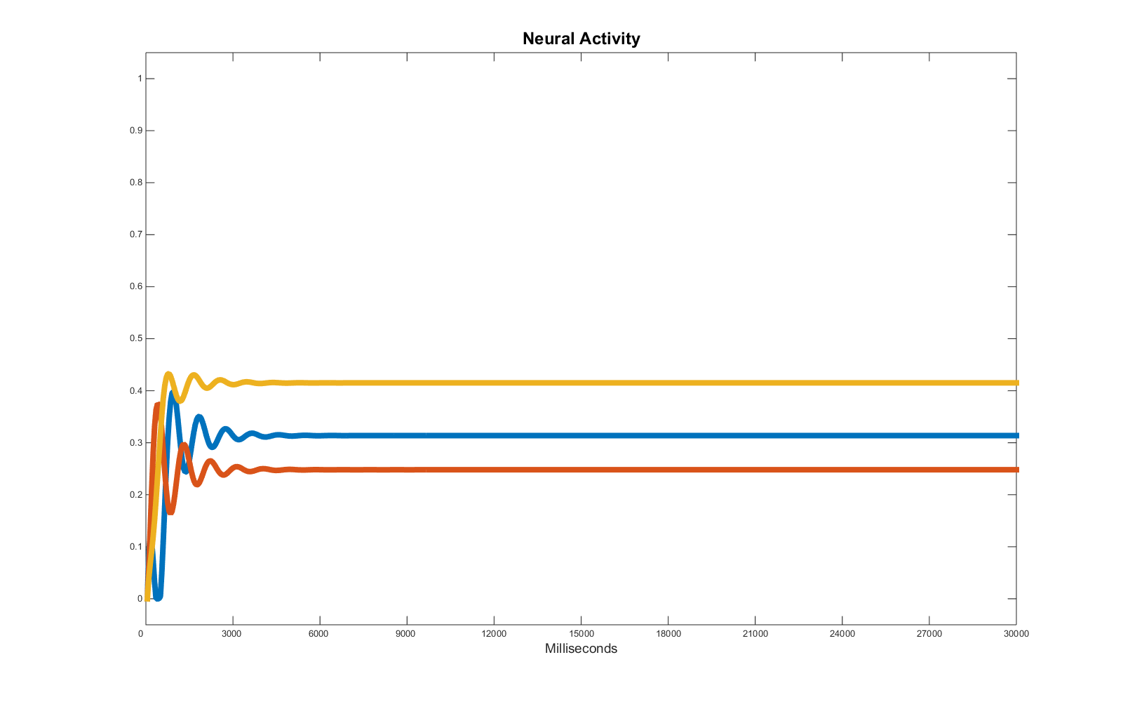
The averaging effect takes the lead and the oscillations are treated like noise. To avoid this problem, we have to change the error function accordingly. The one I propose is as follows:
|
1 2 3 4 5 6 7 8 9 10 11 12 13 14 15 |
%comparison of period, amplitude and centre line of wave functions for n=1:length(output(1,:)) for int=2:4 output_wave=compute_wave(output(:,n), [T/5*int T]); target_wave=compute_wave(target_output(:,n), [T/5*int T]); %comparison: period error=error+abs(target_wave(1)-output_wave(1))^2; %comparison: amplitude error=error+abs((target_wave(2)-output_wave(2))*500)^2; %comparison: centre line distance error=error+abs((target_wave(3)-output_wave(3))*500)^2; %comparison: peak index error=error+abs(target_wave(4)-output_wave(4)); end end |
Having in “compute_wave” (file included in the zip folder) a simple function that extract in the provided interval features such as: wave period, local max and min (ordinates), amplitude, centre line and peak position (abscissa). Since the waves are not constant (the amplitude diminishes), I use the function several times for the same time series (three in the example) in different time intervals, arbitrarily chosen. The weights ascribed to each value comparison have been themselves tuned running the genetic algorithm several times to find a good balance. Consider in this context that distance between target and phenotype is naturally unbalanced in favour of the period (which has a minimum error = 1) in comparison with, e.g., amplitude (which has a maximum error = 1). Hence the mutiplier here used (times 500) for those differences which are otherwise always below 1 in value.
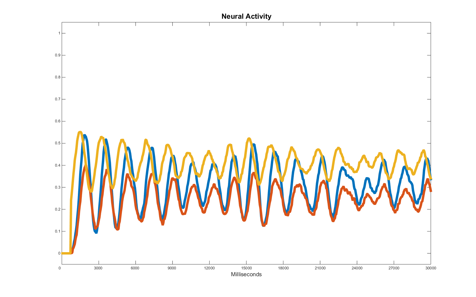
The result looks now more interesting:

But once again, if we analyse the matrix of weights responsible for the target time series and the one selected by the genetic algorithm we will notice important differences:
|
Target parameters |
Optimised parameters |
|
w_11: -0.1310 |
w_11: 0.7787 |
|
w_12: 2.8140 |
w_12: 2.2731 |
|
w_13: -2.0500 |
w_13: 1.5834 |
|
w_21: 1.4760 |
w_21: -0.9940 |
|
w_22: -3.3740 |
w_22: -0.4927 |
|
w_23: -1.2930 |
w_23: 3.3073 |
|
w_31: 2.4480 |
w_31: -1.0431 |
|
w_32: 1.6330 |
w_32: 0.9901 |
|
w_33: 1.0820 |
w_33: -0.0775 |
|
bl1: -1 |
bl1: 0.7522 |
|
bl2: -0.4578 |
bl2: -0.7349 |
|
bl3: 0.9496 |
bl3: -0.8425 |
The whole point of this example is to show that each target requires a specific error function to extract the desired feature and allow a regression specifically focussing on those. So what happens if, like in the previous example, we decide to add noise?
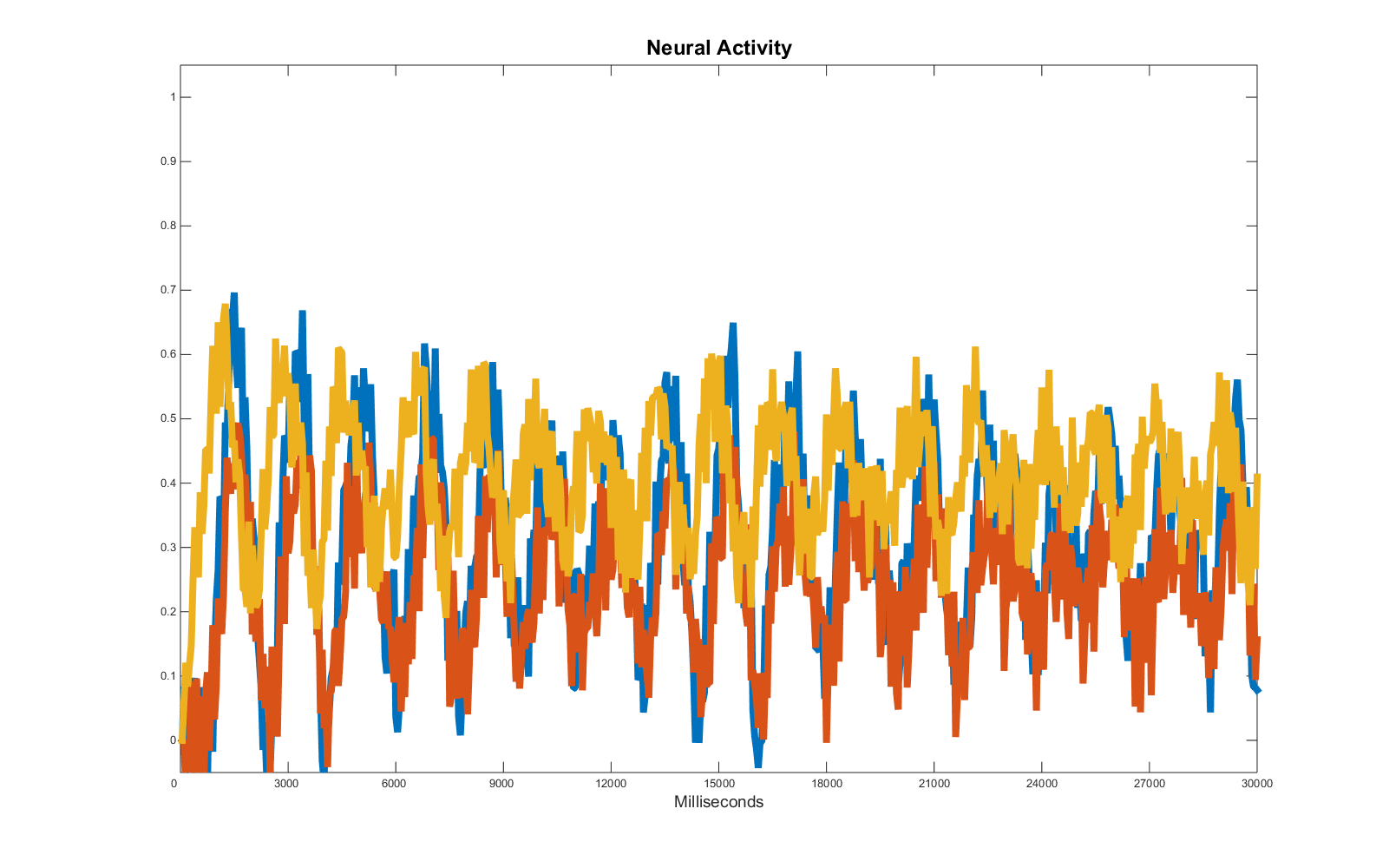
This is an ambiguous case: if we try to replicate all the oscillations, we are entailing we want to replicate the noise as well and there is no (easy) way for the error function to tell the difference between fluctuations caused by noise and fluctuations caused by significant alterations in the activity of the recorded units. Thus, the easiest way to approach the problem is to alter the target data, smoothing the curves and fluctuation until we have once again a pattern we are interested in replicating.
|
1 2 3 4 5 6 7 8 9 |
smooth=15; %average for cluster for ind=smooth:length(all_units.activity(:,1)) noisy_a(ind,:)=sum(all_units.activity(ind-smooth+1:ind,:))/smooth; end all_units.activity=noisy_a; plotting |
This operation result in the following:
Note the ratio noise to signal favours the former in the last part of the target data series as the amplitude of the waves diminishes, whilst the noise range in this case is constant. This effect is detrimental for the regression and has to be weighed accordingly.
Please consider some of these simulations may take several hours, depending on the speed of the processor(s) you are using.
Download all the files here. Regression with genetic algorithms – part 2 (Matlab files)
– Run the genetic algorithm from file GAmain.m
– Check the error function in exp_error
– Run single test to plot the time series using separate_test.m