
It is not surprising that artificial neural networks have been primarily developed as a tool to approximate, estimate and forecast the evolution of time series in the future starting from a dataset describing the past. Indeed, a record of neural activity in a single neuron (spiking) or population (mean field) is just one of the many possible examples of time series.
In this context, the key problem becomes to find a regression tool that might make the network converge towards the simulation of the desired set of target data. Essentialy, a neural network is an approximation tool associating sets of inputs to sets of outputs depending on its implemented function. This function is almost entirely determined by:
- the computation performed in the nodes of the network.
- The architecture of the system (pattern of links in the network).
As a consequence, a good regression tool should find those values for these two features in the neural network that would enable the network to process its input and give back the desired output. Any mathematical or statistical tool is then valid for the regression or optimization of the neural network and will have to face the same problems.
1) the more complex the system used, the wider the space of parameters.
In the present example we will try to optimise different sets of three time series using a neural network composed of 3 nodes (one per time series), 9 links (i.e. fully interconnected) and with a fixed computation per node, but for the basal activity which may also be considered as representing a simplified constant input per unit. In total, “just” 12 parameters. Each parameter increases the space to investigate by an order of magnitude: the key here is the time component required to explore this space to find the optimal solution. Even considering just 12 parameters, a complete exploration with simulations lasting 0.01 seconds each and considering only variations in parameters with steps of 0.1 and range [0 1], would require 0.01 seconds times 10^12 (around 300 years). Long story short, exhaustive exploration à la brute force is out of the picture.
2) the more complex the target time series, the higher the number of required parameters.
In general, as for a polynomial function, there always is a configuration that allows a network to replicate (almost) any numeric series, assuming we can add as many parameters as we want (nodes and/or links), the equivalent of the variable in a polynomial. The problem with this assumption is that it clashes with the first rule in this very short list. As a consequence, it will be necessary to approximate the target data, replicating the features that are considered of the highest importance.
First example.
Let’s consider a simple set of three time series:

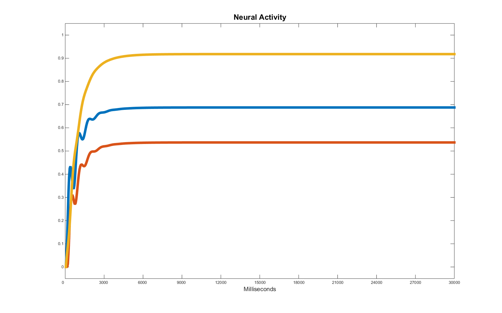
All three units are active at a different level, they reach a steady level (equilibrium point) and it seems this equilibrium is maintained as long as the input is stable. These features entail the system causing them is most likely dominated by attractors, and therefore characterised by high stability. The only feature which creates problems at a first glance is the initial peak of activity of one of the units (in this example, the blue one). That feature may be caused by a variation of the input or by the activity of the other units (e.g. either “red” or “yellow” or both values of activity affect the value of activity of the “blue” unit). In this example, we know any input is caused by the presence of a baseline, so we can positively be sure that the cause of any fluctuation cannot be found in the input variations, as the baselines are constant through the simulation.
The remaining option points towards activity which are dynamically affecting one another. In theory, if we want to forecast how these time series will evolve in the future, it will be necessary to understand the precise causal relations controlling their activity. In practice, it might be sufficient to find any pattern of variables that will enable the system to replicate the equilibrium point, neglecting the initial part of the simulation.
We may want to focus only on the equilibrium state if we assume that the first part of the time series is not informative about the future activity of the units (provided the input will remain constant). In other words, we assume that, if we double the time of the simulation, the stability point will be preserved exactly with the same values we see for most of the target time series. Of course if we also manage to replicate the initial fluctuations, we may have also a plausible hypothesis about the causal relations among the three actors in the play, but this requirement may come at a high price and might not be worth the effort in the present context.
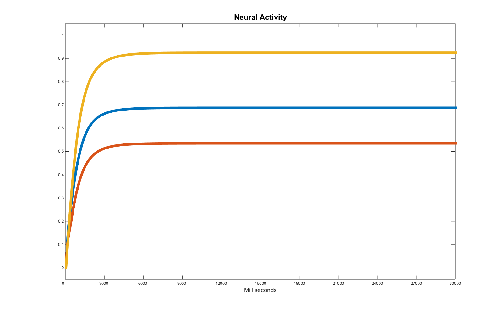
To find the values of the parameters the program uses a genetic algorithm as a regression tool. The selection score is provided by the simple “distance”, point by point, between the output of the neural system and the target time series. As the part of the simulation characterised by the equilibrium state is vastly dominant in terms of data points, any error in determining these values will be considered by the genetic algorithm more important than any error in simulating the first -unstable- part of the time series. So it is not surprising that the selection system manages to optimise the equilibrium state, but significantly fails in replicating the initial part of the time series. Here is the result of the regression via genetic algorithms (options and details in the matlab file: gamain.m):
Of course the problem is that we don’t really know whether we have found a solution which in this specific interval is correctly simulating the vast majority of the target data (score you will usually reach running the program is below 30), but would fail more consistently in the future or if we slightly alter the conditions (e.g. adding an input). As a matter of fact, despite the similarities in the final activities, the set of parameters used to generate the target data strongly differs from the one found by the genetic algorithm, implying significantly different casual relations:
|
Target parameters |
Optimised parameters |
|
w_11: 1 |
w_11: 1.63 |
|
w_12: 0 |
w_12: 4.005 |
|
w_13: 2 |
w_13: 0.306 |
|
w_21: 2 |
w_21: -4.867 |
|
w_22: 0 |
w_22: -2.621 |
|
w_23: 0 |
w_23: 3.841 |
|
w_31: -1 |
w_31: 2.169 |
|
w_32: 0 |
w_32: -0.603 |
|
w_33: 0 |
w_33: -1.607 |
|
bl1: 0 |
bl1: 0.3452 |
|
bl2: 0.6 |
bl2: -0.1938 |
|
bl3: 0.2 |
bl3: 0.7776 |
Yet, the final result successfully predicts the trend of the three time series as we can easily see by prolonging the time of the simulation. In other words, the approximation found by the genetic algorithm represents one of the infinite solutions to the problem of generating the specific equilibrium represented in the target data. The result may look discouraging at first, but the power of the method is clear when we realise it can be used to approximate and extract essential trend features in strongly noisy data. For instance, we can give the genetic algorithm these time series (equivalent of the previous target plus around 20%-30% of noise):

The genetic algorithm, whilst attempting to reduce as much as possible the distance between target time series and the ones produced by randomly generated members of each generation (phenotypes), effectively processes an approximation. In a way the algorithm smooths the curves of the time series, looking for the main trend and ignoring the noise, exposing the hidden equilibrium state. Eventually, the algorithm comes out with a solution of the following type (which establishes yet another of the multiple solutions of this “find the equilibrium” selection).:
Please consider some of these simulations may take several hours, depending on the speed of the processor(s) you are using.
Download all the files here. Regression with genetic algorithms – part 1 (Matlab files)
– Run the genetic algorithm from file GAmain.m
– Check the error function in exp_error
– Run single test to plot the time series using separate_test.m